The joeysvowels package provides a handful of datasets, some subsets of others, that contain formant measurements and other information about the vowels in my own speech. The purpose of the package is to make vowel data easily accessible for demonstrating code snippets when demonstrating working with sociophonetic data.
There are no functions contained in joeysvowels; it’s a data-only package.
Installation
You can install joeysvowels through GitHub:
remotes::install_github("joeystanley/joeysvowels")
You can then load the package like normally:
library(joeysvowels)
Contents
Currently, there are six datasets contained in joeysvowels:
darlais one that was prepared using pretty standard methods, using the DARLA web interface to automatically transcribe, force-align, and extract formants from the audio. The audio was me reading 300 prepared sentences. It’s a bit of a noisy dataset, so it’s a good example of working with real data. It is also very close to the format that FAVE exports its data, so any examples that usedarlacan be easily modified to another FAVE-produced spreadsheet.-
coronalsis a much cleaner, more controlled dataset. You can read about the methods by viewing the documentation (?coronals). Essentially, I read a bunch of (C)CVC(C) nonce words where the consonants were (almost) all coronal. All my vowel phonemes are represented. I aligned and extracted formants from the data myself. Four formants were extracted every 5% of the vowels’ durations, so great for demonstrating functions and visuals involving vowel trajectories.midpointsis a subset ofcoronalsand contains only the midpoints from F1 and F2.mouthis a subset ofcoronalsand is only the MOUTH (/aw/) vowel.mouth_liteis a subset ofmouthand trims away most of the columns and only contains 10 tokens.
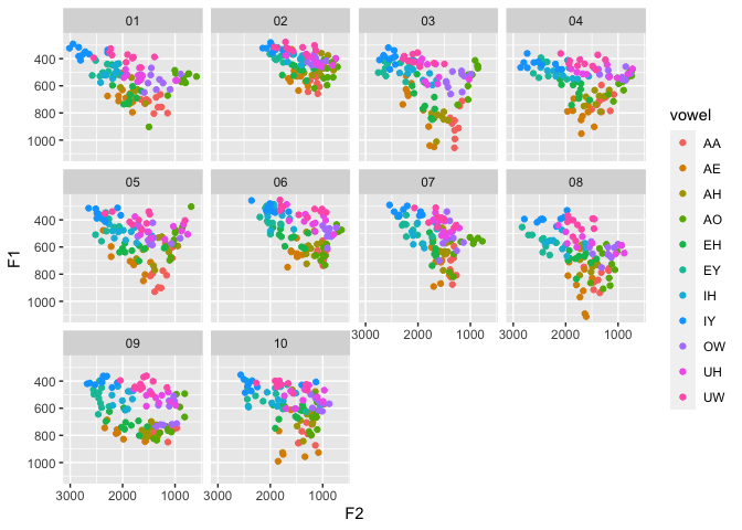
idahoanscontains formant measurements from 11 individuals from the state of Idaho in the US. This is great for testing normalization functions.
Example
You can access the datasets using data(). I’ll briefly visualize the datasets.
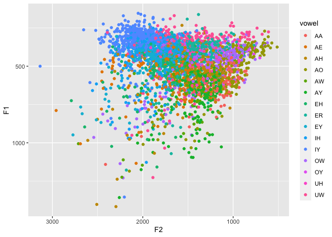
The darla dataset is messy.
data(darla)
ggplot(darla, aes(F2, F1, color = vowel)) +
  geom_point() +
  scale_x_reverse() +
  scale_y_reverse()
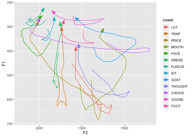
The coronals trajectories show clear influence from the surrounding consonants.
data(coronals)
avg_trajs <- coronals %>%
  group_by(vowel, percent) %>%
  summarize(across(c(F1, F2), mean)) %>%
  print()
## `summarise()` regrouping output by 'vowel' (override with `.groups` argument)

## # A tibble: 273 x 4
## # Groups:   vowel [13]
##    vowel percent    F1    F2
##    <fct>   <dbl> <dbl> <dbl>
##  1 LOT         0  454. 1616.
##  2 LOT         5  592. 1346.
##  3 LOT        10  648. 1283.
##  4 LOT        15  651. 1238.
##  5 LOT        20  661. 1178.
##  6 LOT        25  651. 1176.
##  7 LOT        30  636. 1152.
##  8 LOT        35  630. 1148.
##  9 LOT        40  633. 1153.
## 10 LOT        45  625. 1158.
## # … with 263 more rowsggplot(avg_trajs, aes(F2, F1, color = vowel)) + geom_path(aes(group = vowel), arrow = arrow(angle = 20, length = unit(0.15, "in"), type = "closed")) + scale_x_reverse() + scale_y_reverse()
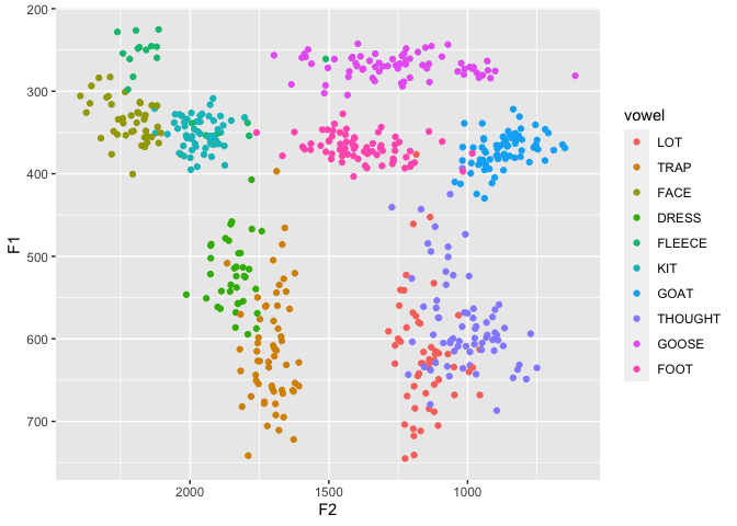
midpoints is pretty clean.
data(midpoints)
ggplot(midpoints, aes(F2, F1, color = vowel)) +
  geom_point() +
  scale_x_reverse() +
  scale_y_reverse()
mouth shows pretty good trajectories.
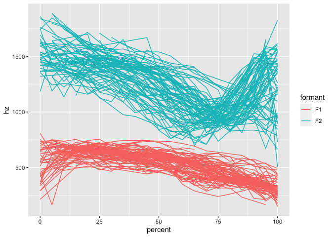
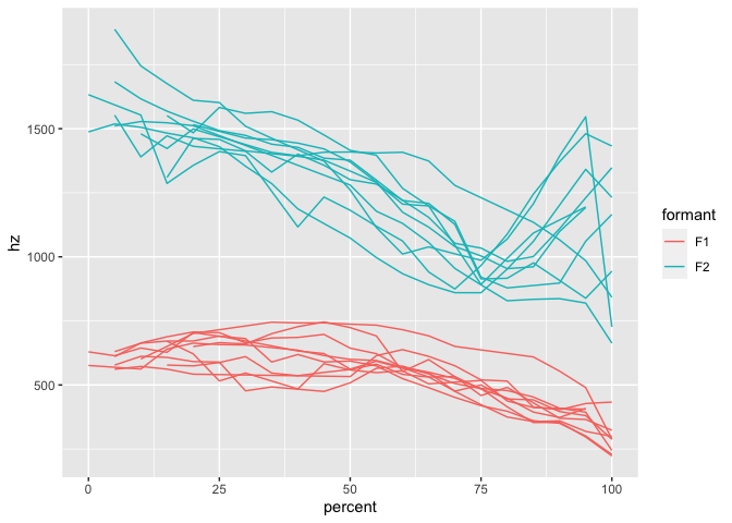
mouth_lite is just smaller.
data(mouth_lite)
ggplot(mouth_lite, aes(percent, hz, color = formant)) +
  geom_path(aes(group = traj_id))
data(idahoans)
ggplot(idahoans, aes(F2, F1, color = vowel)) +
  geom_point() +
  scale_x_reverse() +
  scale_y_reverse() +
  facet_wrap(~speaker)