Convert birth years to generation names.
This package contains functions that will convert years of birth into names of generational cohorts. For example, 1989 becomes "Millennial". The package contains several helper functions to modify the underlying lookup table as well as way to query it.
Installation
The package currently lives on GitHub, so you can install it like you would with any other package on GitHub:
remotes::install_github("joeystanley/generations")
You can then load it like you can with any library.
library(generations)
For the purposes of this tutorial, I’ll load ggplot as well.
Converting years to generations
The main function in this package is generations(). Given a vector of integers, it’ll return a factor of generation names. First, I’ll generate some random years of birth.
I can now easy convert that into generations.
generations(yobs)
##  [1] G.I.       Millennial Gen Z      Silent     G.I.       Lost
##  [7] G.I.       Gen X      Lost       Lost
## Levels: Lost G.I. Silent Gen X Millennial Gen Z
This function works on any year betwen 1435 and 2030. Numbers outside that range return NA.
Note that by default, the function will return the vector as factor, with the levels ordered so that the oldest generation in the vector is first. To get a character vector instead, add the argument as_factor = FALSE.
Customizing output
There are some tweaks you can do to adjust the output of generations(). First, you can return longer forms of the generational names by specifying full_names = TRUE.
generations(yobs, full_names = TRUE)
##  [1] G.I. Generation       Millennial Generation Generation Z
##  [4] Silent Generation     G.I. Generation       Lost Generation
##  [7] G.I. Generation       Generation X          Lost Generation
## [10] Lost Generation
## 6 Levels: Lost Generation G.I. Generation Silent Generation ... Generation Z
What this does is simply add "Generation" to the end of each one, unless it’s "Gen X" (or Y, or Z), in which case it’ll expand it out to simply "Generation X".
You can also show the years included in each generation by adding the years = TRUE argument. This will add a space and, inside a pair of parentheses, the start and end years of that generation, separated by an en dash.
generations(yobs, years = TRUE)
##  [1] G.I. (1908–1928)       Millennial (1984–2007) Gen Z (2008–2030)
##  [4] Silent (1929–1945)     G.I. (1908–1928)       Lost (1886–1907)
##  [7] G.I. (1908–1928)       Gen X (1964–1983)      Lost (1886–1907)
## [10] Lost (1886–1907)
## 6 Levels: Lost (1886–1907) G.I. (1908–1928) ... Gen Z (2008–2030)
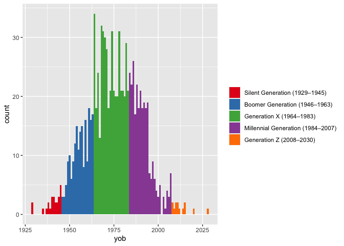
The primary purpose of this is for visualizations, since not everyone is familiar with (or agrees with) the year ranges. For example, if you’ve got a bunch of people and want to visualize the distribution of when they were born, you could have very informative legends.
many_yobs <- tibble(yob = floor(rnorm(1000, 1975, 15))) %>%
  mutate(gen = generations(yob, full_names = TRUE, years = TRUE))
ggplot(many_yobs, aes(yob, fill = gen)) +
  geom_histogram(binwidth = 1) +
  scale_fill_brewer(name = NULL, palette = "Set1")

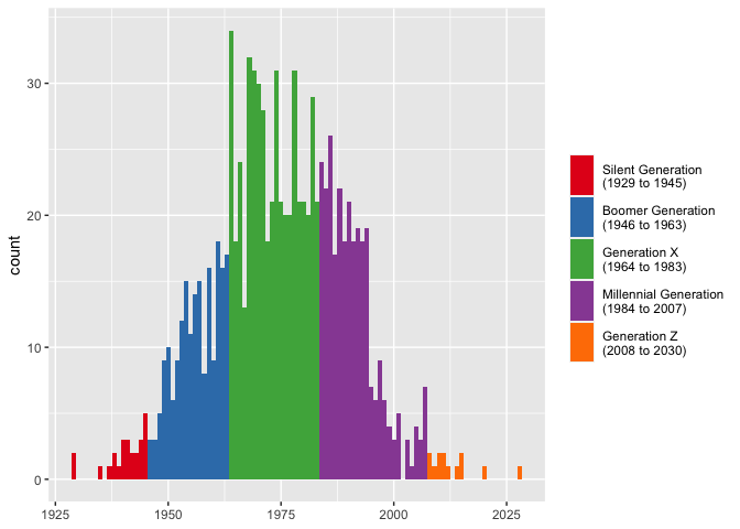
How this additional portion is formatted can be adjusted. If rendering an en dash is troublesome for you, you can change it to something else with years_range_sep. You may also want to change the space between the generation name and the opening parenthesis into a newline character with years_sep, again for visualization purposes.
many_yobs <- many_yobs %>%
  mutate(gen = generations(yob, full_names = TRUE, years = TRUE,
                           years_sep = "\n", years_range_sep = " to "))

ggplot(many_yobs, aes(yob, fill = gen)) +
  geom_histogram(binwidth = 1) +
  scale_fill_brewer(name = NULL, palette = "Set1") +
  labs(x = NULL) +
  theme(legend.key.height = unit(1, "cm"))

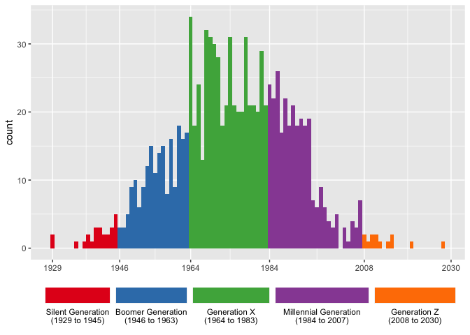
If you want to get really fancy, you can make the legend keys approximate the width they take up on the x-axis and put better tics marks.
widths <- many_yobs %>%
  group_by(gen) %>%
  summarize(width = max(yob) - min(yob)) %>%
  ungroup() %>%
  mutate(width = width / max(width) * 1.4) # you may have to fudge this a little more

ggplot(many_yobs, aes(yob, fill = gen)) +
  geom_histogram(binwidth = 1) +
  scale_fill_brewer(name = NULL, palette = "Set1") +
  scale_x_continuous(breaks = c(1929, 1946, 1964, 1984, 2008, 2030)) +
  labs(x = NULL) +
  theme(legend.position = "bottom") +
  guides(fill = guide_legend(nrow = 1, label.position = "bottom",
                             keywidth = widths$width, default.unit = "inches"))

Querying generation data
To see a list of the generational data, you can use show_generations(), which will return a data frame containing the names, start years, and end years.
##              name start  end
## 1           Gen Z  2008 2030
## 2      Millennial  1984 2007
## 3           Gen X  1964 1983
## 4          Boomer  1946 1963
## 5          Silent  1929 1945
## 6            G.I.  1908 1928
## 7            Lost  1886 1907
## 8      Missionary  1865 1885
## 9     Progressive  1844 1864
## 10         Gilded  1822 1843
## 11 Transcendental  1794 1821
## 12     Compromise  1773 1793
## 13     Republican  1746 1772
## 14        Liberty  1727 1745
## 15      Awakening  1704 1726
## 16  Enlightenment  1675 1703
## 17       Glorious  1649 1674
## 18       Cavalier  1621 1648
## 19        Puritan  1594 1620
## 20  Parliamentary  1569 1593
## 21    Elizabethan  1542 1568
## 22       Reprisal  1517 1541
## 23    Reformation  1497 1516
## 24       Humanist  1459 1496
## 25     Aurthurian  1435 1458
You can also get simple information. For example, if you want to know when the start or end year of a particular generation is, you can use get_start() or get_end():
get_start("Silent")
get_end("Millennial")
You can also find the names of neighboring generations with get_prev_gen() and get_next_gen(), though these were mostly created for internal purposes only rather than for you to use.
get_next_gen("Millennial")
get_prev_gen("Missionary")
Note that if ask for something newer than Gen Z or older than Aurthurian it will return NA.
Customizing generation data
The data that this package uses is loaded as a hidden object when you load the package. You may modify it with the functions described in this section. These changes will affect the dataset so long as the generations package is loaded. You’ll have to reset the data each time to reload it.
The labels and years for each generation are mostly borrowed from Howe & Strauss’ Generational Theory books. However, not everyone agrees on the names and year ranges for the various generations. For this reason, the generations package makes it easy to modify the generations data to your liking.
To rename a generation, use rename_generation(), with the old name first and the new name second. For example, if you want to use Zoomer instead of Gen Z, you can do so.
rename_generation("Gen Z", "Zoomer")
You’ll get a message informing you that the change has been made. If you now run show_generations() you’ll see that the change has been made and if you rerun generations(), you’ll get updated results.
##              name start  end
## 1          Zoomer  2008 2030
## 2      Millennial  1984 2007
## 3           Gen X  1964 1983
## 4          Boomer  1946 1963
## 5          Silent  1929 1945
## 6            G.I.  1908 1928
## 7            Lost  1886 1907
## 8      Missionary  1865 1885
## 9     Progressive  1844 1864
## 10         Gilded  1822 1843
## 11 Transcendental  1794 1821
## 12     Compromise  1773 1793
## 13     Republican  1746 1772
## 14        Liberty  1727 1745
## 15      Awakening  1704 1726
## 16  Enlightenment  1675 1703
## 17       Glorious  1649 1674
## 18       Cavalier  1621 1648
## 19        Puritan  1594 1620
## 20  Parliamentary  1569 1593
## 21    Elizabethan  1542 1568
## 22       Reprisal  1517 1541
## 23    Reformation  1497 1516
## 24       Humanist  1459 1496
## 25 Aurthurian 1435 1458generations(yobs)
##  [1] G.I.       Millennial Zoomer     Silent     G.I.       Lost
##  [7] G.I.       Gen X      Lost       Lost
## Levels: Lost G.I. Silent Gen X Millennial Zoomer
Because many people may want to use the term Zoomer instead of Gen Z, a shortcut function, use_zoomer(), which is just a wrapper around rename_generation("Gen Z", "Zoomer"), is included in the package. The other shortcut functions are use_gen_y(), use_13th(), use_baby_boom() as well as their reciprocals use_gen_z(), use_millennial(), use_gen_x() and use_boomer().
You may also want to change the years. For example, many people consider 1997 as the end of the Millennial Generation. You can make this change with redefine_generation(). With this function, you must specify the new start and the new end year.
redefine_generation("Millennial", 1983, 1997)
## Gen X is now from 1964 to 1982

## Millennial is now from 1983 to 1997

## Zoomer is now from 1998 to 2030
Since changing one generation impacts adjacent generations, you’ll get a message showing you what the new ranges are for this, the previous, and the next generations.
You can reset the data back to its original form with reset_generations().